This is a short demonstration of probabilistic computations in Haskell using a simple implementation of the probability monad.
There are excellent classical papers and blog posts about this topic by Martin Erwig and Steve Kollmansberger, Eric Kidd, Dan Piponi, etc. For serious work you should probably use better libraries like "probability" and "hakaru", available in Hackage.
A random experiment is defined by the probabilities of the elementary outcomes. We can give relative weights that are automatically normalized:
weighted [("hello",1),("hi",3),("hola",1)] :: Prob String
 20.00 % "hello"
 60.00 % "hi"
 20.00 % "hola"
There are shorcuts like bernoulli and uniform with the obvious meaning:
bernoulli (1/5) True False
 80.00 % False
 20.00 % True
coin = uniform ['-','+'] :: Prob Char
coin
 50.00 % '+'
 50.00 % '-'
die = uniform [1..6] :: Prob Int
die
 16.67 % 1
 16.67 % 2
 16.67 % 3
 16.67 % 4
 16.67 % 5
 16.67 % 6
Using standard monad functions and other utilities we can work with probability distributions in a natural and intuitive way.
replicateM 2 die
  2.78 % [1,1]
  2.78 % [1,2]
  2.78 % [1,3]
   ⋮
  2.78 % [6,5]
  2.78 % [6,6]
We could even define a Num instance for distributions, allowing expressions like this
die + die
  2.78 % 2
  5.56 % 3
  8.33 % 4
 11.11 % 5
 13.89 % 6
 16.67 % 7
 13.89 % 8
 11.11 % 9
  8.33 % 10
  5.56 % 11
  2.78 % 12
but we must be careful since some arithmetic equivalences do not hold:
2*die
 16.67 % 2
 16.67 % 4
 16.67 % 6
 16.67 % 8
 16.67 % 10
 16.67 % 12
The operator <-- denotes marginalization:
(!!1) <-- replicateM 3 die
 16.67 % 1
 16.67 % 2
 16.67 % 3
 16.67 % 4
 16.67 % 5
 16.67 % 6
This is based on fmap and normalization, so it works with any projection function:
sum <-- replicateM 2 die
  2.78 % 2
  5.56 % 3
  8.33 % 4
 11.11 % 5
 13.89 % 6
 16.67 % 7
 13.89 % 8
 11.11 % 9
  8.33 % 10
  5.56 % 11
  2.78 % 12
Marginalization of a predicate gives the probability of the corresponding event:
(>4) <-- die
 66.67 % False
 33.33 % True
As suggested by Jaines, small probabilities are better measured in a logarithmic scale:
weighted [(True,10),(False,1)]
  9.09 % False
 90.91 % True
printev $ weighted [(True,10),(False,1)]
True : 10.0 db
printev $ weighted [('A',100),('B',1),('C',0.1)]
'A' : 19.6 db
The operator ! denotes conditioning, which is implemented just by filtering and normalization.
die ! odd
 33.33 % 1
 33.33 % 3
 33.33 % 5
We can combine conditioning and marginalization to calculate the probability of any event in a random experiment. For instance, the distribution of the minimum result of throwing three dice when all results are different is
minimum <-- replicateM 3 die ! (\[a,b,c] -> a/=b && a/=c && b/=c)
 50.00 % 1
 30.00 % 2
 15.00 % 3
  5.00 % 4
The operators (<--) and (!) can be respectively read "of" and "given".
More interesting experiments can be defined using the general rule for the intersection of two events:
$$P(A,B) = P(A|B) P(B)$$
The usual example is the medical test for a certain disease. We assume that the disease occurs in 1 of 1000 people, and the accuracy of the test is 1% for false negatives and 5% for false positives.
disease = bernoulli (1/1000) "ill" "healthy"

test "ill"     = bernoulli (99/100) "+" "-"
test "healthy" = bernoulli (95/100) "-" "+"

med = joint test disease
med
  5.00 % ("+","healthy")
  0.10 % ("+","ill")
 94.90 % ("-","healthy")
  0.00 % ("-","ill")
The two attributes are grouped in a tuple, so marginalization and conditioning
use the selectors fst and snd:
fst <-- med
  5.09 % "+"
 94.91 % "-"
snd <-- med ! ((=="+").fst)
 98.06 % "healthy"
  1.94 % "ill"
The above "query" is not very legible. We could use some helpers to check if the elements of a tuple contain a given value, but in the end using tuples does not scale well:
joint (const coin) (joint (const coin) coin)
 12.50 % ('+',('+','+'))
 12.50 % ('+',('+','-'))
 12.50 % ('+',('-','+'))
 12.50 % ('+',('-','-'))
 12.50 % ('-',('+','+'))
 12.50 % ('-',('+','-'))
 12.50 % ('-',('-','+'))
 12.50 % ('-',('-','-'))
Alternately we can use the more general jointWith to create a more convenient representation for marginalization and conditioning. For example, we can use lists of attributes:
let lcoin = fmap return coin
jointWith (++) (const lcoin) (jointWith (++) (const lcoin) lcoin)
 12.50 % "+++"
 12.50 % "++-"
 12.50 % "+-+"
 12.50 % "+--"
 12.50 % "-++"
 12.50 % "-+-"
 12.50 % "--+"
 12.50 % "---"
Even better, we can use a list of attribute-value pairs to select the variables by name instead of positionally. As an illustration of this technique, the previous medical test experiment is extended to show the evolution of the posterior probabilities given the results of several independent tests. To do this we add attribute names to the above definitions using appropriate helpers:
disease' = setAttr "disease" <-- disease

test' name (attr "disease" -> d) = setAttr name <-- test d

med' = t "t2" . t "t3" . t "t1" $ disease'
  where
    t name = jointWith (++) (test' name)
med'
  0.01 % [("t2","+"),("t3","+"),("t1","+"),("disease","healthy")]
  0.10 % [("t2","+"),("t3","+"),("t1","+"),("disease","ill")]
  0.24 % [("t2","+"),("t3","+"),("t1","-"),("disease","healthy")]
   ⋮
 85.65 % [("t2","-"),("t3","-"),("t1","-"),("disease","healthy")]
  0.00 % [("t2","-"),("t3","-"),("t1","-"),("disease","ill")]
The same conditional probability 'test' works now on attribute lists of different sizes and ordering.
We can now ask any question using a more legible notation:
attr "disease" <-- med' ! "t1" `is` "+"
 98.06 % "healthy"
  1.94 % "ill"
After a second positive it is still more probable to be healthy:
attr "disease" <-- med' ! pos "t1" .&&. pos "t3"
 71.82 % "healthy"
 28.18 % "ill"
But a third independent positive result finally changes the prediction:
attr "disease" <-- med' ! pos "t1" ! pos "t3" ! pos "t2"
 11.40 % "healthy"
 88.60 % "ill"
On the other hand, a single negative result is highly informative, given the low prevalence of the disease:
printev $ attr "disease" <-- med' ! neg "t2"
"healthy" : 49.8 db
attr "disease" <-- med' ! pos "t1" ! pos "t3" ! neg "t2"
 99.59 % "healthy"
  0.41 % "ill"
1) Compute the sum of $n$ dice, where $n$ is the result of throwing a first die. What is the most frequent result?
mdie = joint (\k -> sum <-- replicateM k die) die
This is the marginal distribution of the sum:
mode (fst <-- mdie)
6
2) If a coin comes up heads we throw two dice and add the results, and if the coin comes up tails we throw three dice and get the maximum result:
experr = joint f g
  where
    g = coin
    f '+' = sum     <-- replicateM 2 die
    f '-' = maximum <-- replicateM 3 die
What can we say about the coin from the observed result?
snd <-- experr ! (==1).fst
100.00 % '-'
snd <-- experr ! (==2).fst
 46.15 % '+'
 53.85 % '-'
snd <-- experr ! (==6).fst
 24.79 % '+'
 75.21 % '-'
This is a classical probability puzzle. There is a prize hidden in one of three rooms. You choose one of them. Then they show you one empty room, and give you the opportunity to change your guess to the remaining closed room. Should you stick to your initial guess or it is better to change?
We model it using monadic "do" notation.
monty strategy = do
    prize <- uniform "123"
    guess <- uniform "123"
    open  <- uniform ("123" \\ [guess,prize])
    let final = strategy guess open
    return (prize==final)

stick  g o = g

change g o = head $ "123" \\ [g,o]
monty stick
 66.67 % False
 33.33 % True
monty change
 33.33 % False
 66.67 % True
The optimal strategy is easily understood in a more general problem, with a very high number of rooms $n$, and after your initial guess they open $n-2$ empty rooms.
This is a beautiful problem discussed by Allen Downey.
We assume that a child can be a boy or a girl with equal probability:
natural :: Prob String
natural = bernoulli (1/2) "Boy" "Girl"
Children names follow some distribution, for example:
name :: String -> Prob String

name "Boy" = weighted [("N1",6),("N2",4)]
name "Girl" = weighted [("N3",4),("N4",4),("N5",2)]
Then, the distribution of name and sex for a child is
let child = joint name natural
child
 30.00 % ("N1","Boy")
 20.00 % ("N2","Boy")
 20.00 % ("N3","Girl")
 20.00 % ("N4","Girl")
 10.00 % ("N5","Girl")
We are actually interested in families with two children:
let family = replicateM 2 child
family
  9.00 % [("N1","Boy"),("N1","Boy")]
  6.00 % [("N1","Boy"),("N2","Boy")]
  6.00 % [("N1","Boy"),("N3","Girl")]
  6.00 % [("N1","Boy"),("N4","Girl")]
   ⋮
  2.00 % [("N5","Girl"),("N3","Girl")]
  2.00 % [("N5","Girl"),("N4","Girl")]
  1.00 % [("N5","Girl"),("N5","Girl")]
We define some helpers:
let names = map fst
names <-- family
  9.00 % ["N1","N1"]
  6.00 % ["N1","N2"]
  6.00 % ["N1","N3"]
  6.00 % ["N1","N4"]
   ⋮
  2.00 % ["N5","N3"]
  2.00 % ["N5","N4"]
  1.00 % ["N5","N5"]
let sexes = map snd
sexes <-- family
 25.00 % ["Boy","Boy"]
 25.00 % ["Boy","Girl"]
 25.00 % ["Girl","Boy"]
 25.00 % ["Girl","Girl"]
Our first question is: what is the probability that the two children are girls, given that the first child is a girl?
let girl = (=="Girl") . snd
let first p = p . head
sexes <-- family ! first girl
 50.00 % ["Girl","Boy"]
 50.00 % ["Girl","Girl"]
all girl <-- family ! first girl
 50.00 % False
 50.00 % True
The sex of the second child is obviously not influenced by the fact that the first child is a girl.
The second question is: what is the probability that the two children are girls, given that any of the children is a girl?
sexes <-- family ! any girl
 33.33 % ["Boy","Girl"]
 33.33 % ["Girl","Boy"]
 33.33 % ["Girl","Girl"]
all girl <-- family ! any girl
 66.67 % False
 33.33 % True
In this case only one of the 4 combinations is discarded by the condition, so the probability reduces to 1/3.
Until now the names of the children have played no role and have been marginalized out in the computations. The really interesting question in this puzzle is the following:
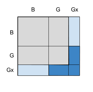
What is the probability that the two children are girls, given that any of the children is a girl named Florida?
We denote this special name as "N5". (There is nothing special about names, the key point in this problem is that the conditioning event includes an additional property.) This new condition can be expressed as:
all girl <-- family ! any (==("N5" , "Girl"))
 52.63 % False
 47.37 % True
Depending on the size of the probability of this additional property, the result increases towards 1/2, as if the first child is known for sure to be a girl. This is initially counterintuitive since the name of a child should not affect the sex of the other one. The best way to explain the result is this figure taken from the blog post:
With this particular distribution of names we have
any (==("N5" , "Girl")) <-- family
 81.00 % False
 19.00 % True
all girl .&&. any (==("N5" , "Girl")) <-- family
 91.00 % False
  9.00 % True
9/19
0.47368421052631576
The above examples involve simple discrete distributions that can be computed by exhaustive search. Realistic problems with high dimensional continuous random variables, infinite recursive experiments, etc., require more advanced techniques.