Bayesian inference

This is a simple example of Bayesian inference using the Metropolis algorithm.

We start from a sample of size 10 taken from a normal density with $\mu=1$ and $\sigma = 1/2$. The sample mean is 1.09 and the sample std is 0.55.


 1 
 2 
 3 
 4 
 5 
 6 
 7 
 8 
 9 
 10 

 sample # 


 -4 
 -3 
 -2 
 -1 
 0 
 1 
 2 
 3 
 4 


 value 


only $\mu$

First we estimate the posterior distribution of the mean when σ is known (and uniform prior):


 -2 
 -1 
 0 
 1 
 2 

 μ 


 0.0 
 0.2 
 0.4 
 0.6 
 0.8 
 1.0 
 1.2 
 1.4 
 1.6 
 1.8 
 2.0 
 2.2 
 2.4 
 2.6 


 p(μ) 


 p(μ|D) 


 0.75 


 1.40 


(Acceptance ratio: 0.1896 )

The mean and std of the posterior mean is consistent with what we expect: 1.09, 0.16 , and $\sigma/\sqrt n = 0.16$.

We also show a 96% credible interval in the histograms.

only $\sigma$

Now we compute the posterior σ for known μ, in this case using the noninformative prior $\sigma^{ -1 }$:


 0.0 
 0.5 
 1.0 
 1.5 
 2.0 
 2.5 
 3.0 

 σ 


 0 
 1 
 2 
 3 
 4 


 p(σ) 


 p(σ|D) 


 0.36 


 0.90 


(Acceptance ratio: 0.156 )

$\mu$ and $\sigma$

If nothing is known about the parameters we get slightly heavier tails:


 -3 
 -2 
 -1 
 0 
 1 
 2 
 3 

 μ 


 0.0 
 0.2 
 0.4 
 0.6 
 0.8 
 1.0 
 1.2 
 1.4 
 1.6 
 1.8 
 2.0 
 2.2 


 p(μ) 


 p(μ|D) 


 0.66 


 1.50 


 0.0 
 0.5 
 1.0 
 1.5 
 2.0 
 2.5 
 3.0 

 σ 


 0 
 1 
 2 
 3 


 p(σ) 


 p(σ|D) 


 0.33 


 0.93 


(Acceptance ratio: 0.1327 , with $\sigma_m = 0.3$).

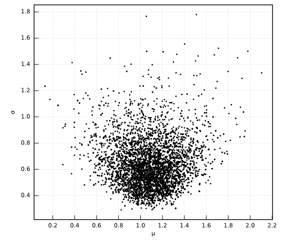
This is the joint distribution of $(\mu,\sigma)$:

plot2c

outliers

We add a few outliers:


 2 
 4 
 6 
 8 
 10 
 12 

 sample # 


 -4 
 -3 
 -2 
 -1 
 0 
 1 
 2 
 3 
 4 


 sample value 


If we use a simple Gaussian model the estimated posterior distributions obviously have large dispersion:


 -3 
 -2 
 -1 
 0 
 1 
 2 
 3 

 μ 


 0.0 
 0.1 
 0.2 
 0.3 
 0.4 
 0.5 
 0.6 
 0.7 
 0.8 


 p(μ) 


 p(μ|D) 


 -0.60 


 1.80 


 0.0 
 0.5 
 1.0 
 1.5 
 2.0 
 2.5 
 3.0 
 3.5 
 4.0 
 4.5 
 5.0 

 σ 


 0.0 
 0.2 
 0.4 
 0.6 
 0.8 
 1.0 


 p(σ) 


 p(σ|D) 


 1.30 


 3.05 


(Acceptance ratio: 0.3877 , with $\sigma_m = 0.5$).

A better model for this kind of data is a mixture of normal ($\mu$,$\sigma$) with weight $(1-p)$ and a much wider normal (0,5) with weight $p$. We set a uniform prior on $p$.

The result is quite good: the posterior $\mu$ and $\sigma$ are similar to the case with clean data:


 -3 
 -2 
 -1 
 0 
 1 
 2 
 3 

 μ 


 0.0 
 0.2 
 0.4 
 0.6 
 0.8 
 1.0 
 1.2 
 1.4 
 1.6 
 1.8 


 p(μ) 


 p(μ|D) 


 0.54 


 1.68 


 0.0 
 0.5 
 1.0 
 1.5 
 2.0 
 2.5 
 3.0 

 σ 


 0.0 
 0.2 
 0.4 
 0.6 
 0.8 
 1.0 
 1.2 
 1.4 
 1.6 
 1.8 
 2.0 
 2.2 
 2.4 
 2.6 
 2.8 
 3.0 


 p(σ) 


 p(σ|D) 


 0.24 


 1.41 


The posterior distribution of the ratio of outliers shows that this ratio is around 0.3, although a precise value cannot be determined from this sample size.


 0.0 
 0.2 
 0.4 
 0.6 
 0.8 
 1.0 

 p 


 0 
 1 
 2 
 3 


 p(p) 


 p(p|D) 


 0.07 


 0.66 


(Acceptance ratio: 0.2034 , with $\sigma_m = 0.02$).

robustness

If we use this robust model with the initial "clean" data we get the following result:


 -3 
 -2 
 -1 
 0 
 1 
 2 
 3 

 μ 


 0.0 
 0.2 
 0.4 
 0.6 
 0.8 
 1.0 
 1.2 
 1.4 
 1.6 
 1.8 
 2.0 
 2.2 


 p(μ) 


 p(μ|D) 


 0.66 


 1.50 


 0.0 
 0.5 
 1.0 
 1.5 
 2.0 
 2.5 
 3.0 

 σ 


 0 
 1 
 2 
 3 


 p(σ) 


 p(σ|D) 


 0.33 


 0.96 


From a naive machine learning viewpoint it is quite remarkable that the intervals estimated by this richer model are only slightly wider than those obtained by the simpler normal model.

The posterior distribution of the ratio of outliers that we get in this case (which can be considered as a nuisance parameter) shows that the outliers are unlikely now, but again they cannot be ruled out from this small sample.


 0.0 
 0.2 
 0.4 
 0.6 
 0.8 
 1.0 

 p 


 0 
 1 
 2 
 3 
 4 
 5 
 6 
 7 
 8 
 9 


 p(p) 


 p(p|D) 


 0.00 


 0.31 


The shape of this distribution is qualitatively different now. As the sample size increases, the probability mass of the ratio of outliers moves to the left (towards $p=0$), but since samples from the outlier distribution can also appear in the region of the clean data we will always obtain a small tail over $p>0$.

In any case, the marginal distributions for $\mu$ and $\sigma$ provide excellent estimations without any overfitting.

(Acceptance ratio: 0.1735 , with $\sigma_m = 0.05$).

curve fitting

(in construction)

concluding remarks

The power of the Bayesian approach, working from such basic principles, is impressive. In combination with Metropolis and other sampling algorithms we can solve interesting and nontrivial problems using a few lines of code.